Principal Component Analysis (PCA) is arguably the most fundamental dimensionality reduction technique. In this post, I cover five important practical applications of PCA, including some that are not very obvious, and illustrate them using published research or with examples of my own.
My goal is to build the intuition for recognizing when PCA is the right tool, so the review of the method itself is deliberately brief—most of the post is the use cases. If you already know PCA, feel free to skip straight to the “Uses of PCA” section.
Throughout this post, some code blocks are folded by default. These are blocks whose contents are not central to the point being made—setup boilerplate, helper functions, or longer plotting code that would otherwise interrupt the flow. They are included for completeness and can be expanded at any time. The first block below is one such example: it loads packages and defines shared helpers (a plot theme, a color palette, and a few small utility functions) used throughout the post.
Setup: packages, theme, palette, and helper functions
library(readr)library(tidyr)library(dplyr, warn.conflicts =FALSE)library(ggplot2)library(ggrepel)library(GGally)library(patchwork)library(knitr)library(sessioninfo)# Shared theme applied to every plot in the posttheme_set(theme_minimal(base_size =12))# Shared palette, referenced by name instead of color literalspal <-list(point ="steelblue", # observations / primary seriesaccent ="firebrick", # loadings / negative values / baselinesneutral ="grey60"# reference lines)# Colorblind-safe (Okabe-Ito) palette for categorical color/fill scales.# Yellow (#F0E442) is moved last: it has poor contrast on a white background,# so it is only reached when a plot needs more than seven categories.okabe_ito <-c("#E69F00", "#56B4E9", "#009E73", "#0072B2","#D55E00", "#CC79A7", "#999999", "#F0E442")# Percent of total variance explained by each principal componentvar_explained <-function(pca) 100* pca$sdev^2/sum(pca$sdev^2)# Axis label like "PC1 (75.0%)" for the i-th principal componentpc_label <-function(pca, i) sprintf("PC%d (%.1f%%)", i, var_explained(pca)[i])# Reverse scale(): multiply each column by its SD, then add its meanunscale <-function(x, means, sds) {sweep(sweep(x, 2, sds, "*"), 2, means, "+")}
One more note: plots in this post are built with either custom ggplot2 code or pre-packaged ggplot2 code—which is the case in GGally::ggpairs—rather than R’s built-in plotting functions (biplot, pairs, screeplot, and so on). There is nothing wrong with those functions—base R versions are often quicker and perfectly adequate. The custom code is purely a personal preference for visual consistency and style across the post.
A related note on tables: the styling difference between them is intentional. When the point is to show what an R object actually looks like—the raw structure a function hands back—I print it as-is. When I have assembled a summary table to make a particular point, I format it with knitr::kable(). So the two styles are a cue for which of the two you are looking at.
What PCA does to your data
You have a data frame with \(p\) columns and \(n\) rows. PCA constructs \(p\) new columns from the data. Strictly speaking, it is \(\min(n-1, p)\) columns, but in most practical applications \(n\) is much greater than \(p\), so this is just \(p\).
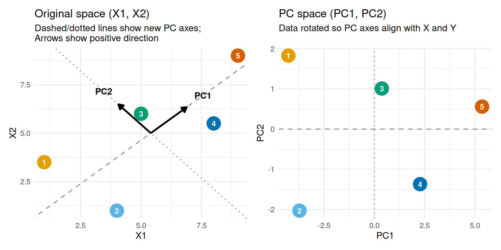
The quickest way to see what this means is on a tiny example: five points with two columns, \(X_1\) and \(X_2\), shown before and after PCA.
cx <-mean(orig$X1)cy <-mean(orig$X2)L <- pca_result$rotation # each column is a loading vectorslope1 <- L[2, 1] / L[1, 1]intercept1 <- cy - slope1 * cxslope2 <- L[2, 2] / L[1, 2]intercept2 <- cy - slope2 * cxarrow_len <-2.0p1 <-ggplot(orig_tbl, aes(x = X1, y = X2, color =factor(Point))) +geom_abline(slope = slope1, intercept = intercept1,color = pal$neutral, linetype ="dashed", linewidth =0.7) +geom_abline(slope = slope2, intercept = intercept2,color = pal$neutral, linetype ="dotted", linewidth =0.7) +annotate("segment",x = cx, y = cy,xend = cx + L[1, 1] * arrow_len,yend = cy + L[2, 1] * arrow_len,arrow =arrow(length =unit(0.25, "cm"), type ="closed"),color ="black", linewidth =1.1) +annotate("segment",x = cx, y = cy,xend = cx + L[1, 2] * arrow_len,yend = cy + L[2, 2] * arrow_len,arrow =arrow(length =unit(0.25, "cm"), type ="closed"),color ="black", linewidth =1.1) +geom_point(size =8) +geom_text(aes(label = Point), color ="white", fontface ="bold", size =3.5) +annotate("text",x = cx + L[1, 1] * (arrow_len +0.9),y = cy + L[2, 1] * (arrow_len +0.9),label ="PC1", fontface ="bold", size =4) +annotate("text",x = cx + L[1, 2] * (arrow_len +0.9),y = cy + L[2, 2] * (arrow_len +0.9),label ="PC2", fontface ="bold", size =4) +scale_color_manual(values = okabe_ito) +labs(title ="Original space (X1, X2)",subtitle ="Dashed/dotted lines show new PC axes;\nArrows show positive direction",x ="X1", y ="X2") +theme(legend.position ="none")p2 <-ggplot(pcs_tbl, aes(x = PC1, y = PC2, color =factor(Point))) +geom_hline(yintercept =0, color = pal$neutral, linetype ="dashed", linewidth =0.7) +geom_vline(xintercept =0, color = pal$neutral, linetype ="dotted", linewidth =0.7) +geom_point(size =8) +geom_text(aes(label = Point), color ="white", fontface ="bold", size =3.5) +scale_color_manual(values = okabe_ito) +labs(title ="PC space (PC1, PC2)",subtitle ="Data rotated so PC axes align with X and Y\n",x ="PC1", y ="PC2") +theme(legend.position ="none")p1 | p2
In the right panel the point cloud has simply been rotated: PC1 and PC2 are new axes drawn through the data, and each point’s coordinates along them are its principal component scores. It is also common to refer to the new columns simply as principal components and to use PC1, PC2, up to the \(p\)th to refer to each of these new transformed columns. I will also be doing this.
Each principal component is a linear combination of the original columns. Following the notation in James et al. (2021), the first is
where the \(\phi\)’s are the loadings. They are not arbitrary—they are chosen to satisfy a few properties, and it is those properties that make PCA useful in everything that follows:
PC1 has the largest variance possible, subject to its loadings having unit norm (\(\sum_{j} \phi_{j1}^2 = 1\), a constraint that simply stops the variance from being inflated by scaling the loadings up).
Each later component has the largest variance possible while staying orthogonal to all the earlier ones. So PC2 has less variance than PC1, PC3 less than PC2, and so on down to the last. The loading vectors end up mutually perpendicular and unit-length—orthonormal.
The new columns are mutually uncorrelated.
We start with \(p\) columns and end with \(p\) columns, so on its face this is not dimensionality reduction. The reduction comes from the ordering: PC1 carries the most variance and each component after it carries less. Reduction happens when we keep only the first \(M\) components (\(M < p\)) and ask how much of the data they still represent—which, as we will see, can be most of it.
Example: World Bank World Development Indicators
World Bank World Development Indicators provide a wide range of, well, development indicators, for countries or country-like entities around the world. For this example, I pulled 7 of them for 2023. These are:
Fertility rate, total (births per woman)
GDP per capita, PPP (constant 2021 international $)
Mortality rate, infant (per 1,000 live births)
Life expectancy at birth, total (years)
Access to electricity (% of population)
Urban population (% of total population)
Individuals using the Internet (% of population)
Because their API is not working the best, I went to their website, manually downloaded a CSV file and cleaned it. You can can download the cleaned CSV file here. Here, I drop any rows where any value is missing—i.e. I only retain the countries whose values for all 7 variables are available. Then, we take a look at the data.
df <-read_csv("wb2023.csv", show_col_types =FALSE) |>drop_na()print(df, width =200, n =6)
Here, the numeric data we want to transform lives in all the columns other than country_name. So let’s separate that part out.
data <- df |>select(-country_name)
Before we proceed, why is this a good data set to illustrate PCA? One of the features of development is that various aspects of development are going to tend to go hand in hand—most people understand this intuitively. Higher income countries are going to tend to have lower infant mortality rates, higher life expectancy, more people using the internet, and so on. This does not mean a one to one overlap and this does not mean individual dimensions do not contribute any new information. In fact, when individual cases or groups of cases deviate from a general trend like this, it can be an interesting subject of study of its own—for example, countries that are rich generally tend to be democratic, except for countries that are rich mainly because of natural resources—those are studied under the term “resource curse.”
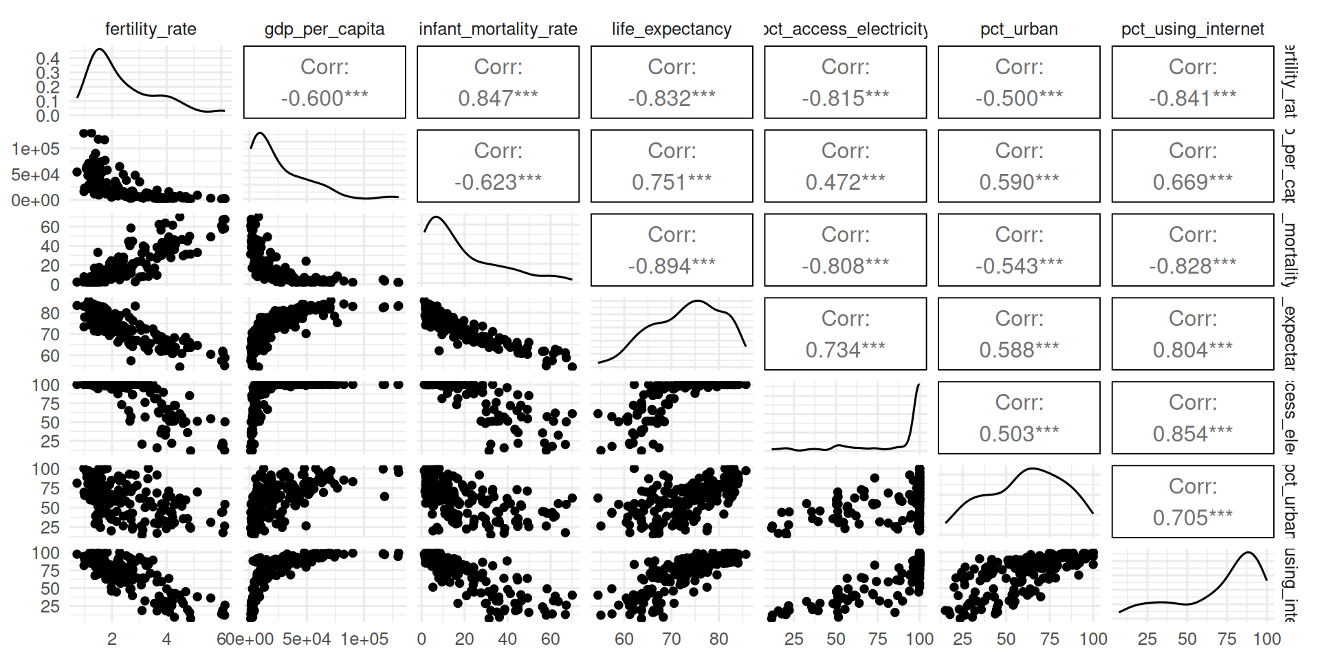
For the World Bank data, let’s see that our intuition about the correlations between individual features does match reality:
ggpairs(data)
Pairwise scatter plots confirm what we expect—that a lot of the variables in the data are highly correlated. Tangentially, the “L” shape relationship the GDP per capita has with other variables shows that we would get even higher correlation—and better dimensionality reduction—by logging that variable, but we will hold off on that here.
Before running PCA it is recommended practice to scale the data: for each variable, subtract the mean and then divide by its standard deviation so that every column ends up with mean 0 and variance 1. This matters because our variables arrive on wildly different scales—compare their variances before and after scaling:
Without scaling, variance maximization leans on whichever variables happen to have the largest variance, placing the highest loadings on them. That makes the result depend on arbitrary unit choices—whether GDP per capita is in US Dollars or Japanese Yen, whether life expectancy is in years or months—even though those choices carry no real information. Scaling removes that dependence by putting every variable on equal footing. Subtraction of the mean is equally important, but I will not expand on that here.
NoteScaling does not imply normality
Scaling has nothing to do with whether a variable is normally distributed. A scaled variable has mean 0 and variance 1, but that does not make it normal—you can scale a binary variable, which is not remotely normal, and it will still have mean 0 and variance 1.
Okay, we can now run PCA with prcomp()
pca <- data_scaled |>prcomp()
The object we get contains two objects that are important:
A rotation matrix that contains the loadings:
pca$rotation |>round(3) # you really don't need more decimals do you?
We can now trace the whole cycle. The original columns had wildly different variances; scaling equalized them to a variance of 1 each, for a total of 7; PCA then redistributes that same total of 7 across the new columns, ordered from the largest variance to the smallest. The table below shows each component’s variance next to its share of that total:
pc_var <-apply(pca$x, 2, var)data.frame(Variance = pc_var,Share =var_explained(pca),row.names =names(pc_var)) |>kable(digits =2, col.names =c("Variance", "Share of total (%)"))
Variance
Share of total (%)
PC1
5.27
75.31
PC2
0.71
10.10
PC3
0.48
6.92
PC4
0.22
3.10
PC5
0.16
2.22
PC6
0.09
1.31
PC7
0.07
1.05
This shows something important: in this dataset, the first principal component alone captures 75% of the total variance—a single dimension represents most of the information in the data. It bears repeating that this does not mean the remaining dimensions are empty: it is 75%, not 100%.
For this to become dimensionality reduction, we keep some of these columns and not others—the ones with the most variance, say the first two or the first five. Equivalently, it is a decision about how many columns from the end to discard.
Visualizing PCA
PCA has two standard visualizations: the biplot and the scree plot.
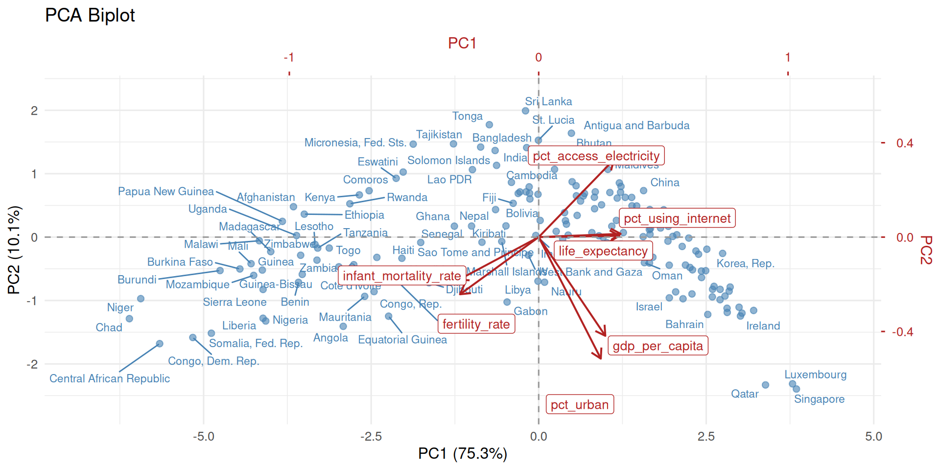
A biplot displays the observations and the variables in the same figure, using the first two principal components—the two highest-variance ones that still fit in a 2D plot. It is a workhorse of exploratory data analysis.
Show biplot helper function
biplot_ggplot <-function(pca, pc_x =1, pc_y =2, labels =NULL, scale =1) {# --- Extract scores (observations) --- scores <-as.data.frame(pca$x[, c(pc_x, pc_y)])colnames(scores) <-c("PC_x", "PC_y")# --- Extract loadings (variables) --- loadings <-as.data.frame(pca$rotation[, c(pc_x, pc_y)])colnames(loadings) <-c("PC_x", "PC_y") loadings$variable <-rownames(loadings)# --- Apply scale: mirrors biplot.prcomp exactly ---# lam = sdev * sqrt(n), then raised to `scale` power.# Scores are divided by lam; loadings are multiplied by lam.# scale=1 → Gabriel biplot (loadings interpretable as correlations);# scale=0 → preserves raw scores and raw loadings (ISLR convention). lam <- pca$sdev[c(pc_x, pc_y)] *sqrt(nrow(pca$x))if (scale <0|| scale >1) warning("'scale' is outside [0, 1]") lam <-if (scale !=0) lam^scale elsec(1, 1) scores$PC_x <- scores$PC_x / lam[1] scores$PC_y <- scores$PC_y / lam[2] loadings$PC_x <- loadings$PC_x * lam[1] loadings$PC_y <- loadings$PC_y * lam[2]# --- Ratio for secondary axes: mirrors biplot.default ---# The loading coordinate space spans `ratio` times the score space,# so loadings are plotted at loading/ratio in score coordinates.# The top/right axes then label those positions with loading values. unsigned_range <-function(x) c(-abs(min(x, na.rm =TRUE)), abs(max(x, na.rm =TRUE))) rangx <-range(unsigned_range(scores$PC_x), unsigned_range(scores$PC_y)) ratio <-max(unsigned_range(loadings$PC_x) /unsigned_range(scores$PC_x),unsigned_range(loadings$PC_y) /unsigned_range(scores$PC_y) )# Loadings mapped into score coordinate space for plotting.# Arrows end at 0.8× (same as base R); labels sit at the full tip. loadings$arr_x <- loadings$PC_x *0.8/ ratio loadings$arr_y <- loadings$PC_y *0.8/ ratio loadings$tip_x <- loadings$PC_x / ratio loadings$tip_y <- loadings$PC_y / ratio# --- Axis limits: tight around plotted data with a small buffer ---# Computed independently per axis so the y viewport is not padded out to# match the x extent (which is the effect of the shared `rangx` approach). buf <-0.07 xlim_plot <-range(c(scores$PC_x, loadings$tip_x)) ylim_plot <-range(c(scores$PC_y, loadings$tip_y)) xlim_plot <- xlim_plot +diff(xlim_plot) *c(-buf, buf) ylim_plot <- ylim_plot +diff(ylim_plot) *c(-buf, buf)# --- Variance explained for primary axis labels --- x_lab <-pc_label(pca, pc_x) y_lab <-pc_label(pca, pc_y)# --- Plot ---ggplot() +# Observation scoresgeom_point(data = scores, aes(PC_x, PC_y),color = pal$point, alpha =0.6, size =2) +# Score labels (optional) { if (!is.null(labels))geom_text_repel(data = scores, aes(PC_x, PC_y, label = labels),color = pal$point, size =3, max.overlaps =15) } +# Loading arrows (drawn 80% of the way, matching base R)geom_segment(data = loadings,aes(x =0, y =0, xend = arr_x, yend = arr_y),arrow =arrow(length =unit(0.3, "cm")),color = pal$accent, linewidth =0.7) +# Variable labels at full tip positiongeom_label_repel(data = loadings,aes(tip_x, tip_y, label = variable),color = pal$accent, size =3.5) +geom_hline(yintercept =0, linetype ="dashed", color = pal$neutral) +geom_vline(xintercept =0, linetype ="dashed", color = pal$neutral) +# Primary axes (scores) + secondary axes (loadings) on top and right.# sec_axis(~ . * ratio) converts a score-space position back to a loading value.scale_x_continuous(name = x_lab,limits = xlim_plot,sec.axis =sec_axis(~ . * ratio, name =sprintf("PC%d", pc_x)) ) +scale_y_continuous(name = y_lab,limits = ylim_plot,sec.axis =sec_axis(~ . * ratio, name =sprintf("PC%d", pc_y)) ) +labs(title ="PCA Biplot") +theme(axis.text.x.top =element_text(color = pal$accent),axis.text.y.right =element_text(color = pal$accent),axis.title.x.top =element_text(color = pal$accent),axis.title.y.right =element_text(color = pal$accent),axis.ticks.x.top =element_line(color = pal$accent),axis.ticks.y.right =element_line(color = pal$accent) )}
What do we see in this plot? There is one arrow representing each variable—and the axes at the top and right show how much that variable contributes to PC1 and PC2, i.e. its loadings. For example, we can observe that the highest contributors to the first principal component are pct_using_internet and life_expectancy. In addition to those two, gdp_per_capita, pct_urban, and pct_access_electricity all contribute positively to the first principal component, although they are a bit smaller in absolute value. This means that higher values of all of five of these variables—for example, more per capita income, more life expectancy, and more internet access—will be associated with higher scores on PC1. The variables infant_mortality_rate and fertility_rate, on the other hand, negatively contribute to PC1. The higher a country’s values are on these two variables, the lower their PC1 score is going to tend to be.
In the other two axes, we see PC1 and PC2 scores for individual observations. We can already see here how PC1 can be seen as a single number “summary” of a country’s level of development. So, from the plot, we can quickly see which countries are the most and least developed based on this crude and quick metric by reading their PC1 scores on the X-axis.
ImportantLoadings are unique only up to sign
PCA loadings are unique only up to sign: multiplying a component’s loadings by (-1) gives an equally valid solution (and that would flip the signs of the principal component scores as well.) So, in an example like this, you would need to check what direction actually represents “higher” or “lower” development. If you wanted, you could multiply it by -1 after the fact if the higher values of the principal components do not correspond to what you would intuitively expect.
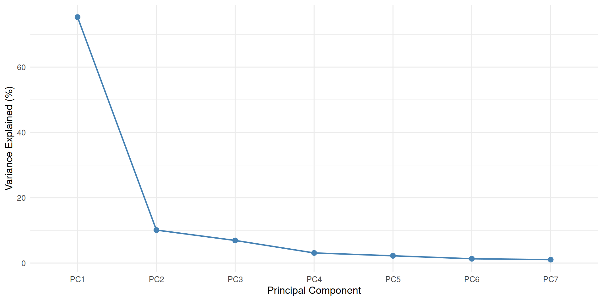
The second plot often produced for PCA is a scree plot, which is a visual way of representing the share of variance captured by each principal component.
Show screeplot helper function
screeplot_ggplot <-function(pca) { ve <-var_explained(pca) scree_df <-data.frame(pc =factor(paste0("PC", seq_along(ve)),levels =paste0("PC", seq_along(ve))),var_explained = ve )ggplot(scree_df, aes(x = pc, y = var_explained)) +geom_line(aes(group =1), color = pal$point, linewidth =0.8) +geom_point(color = pal$point, size =2.5) +labs(x ="Principal Component", y ="Variance Explained (%)")}
screeplot_ggplot(pca)
Uses of PCA
I will highlight five uses of PCA that I find especially useful.
Preprocessing for Clustering
Preprocessing for Supervised Learning
Index Construction
Comparing Effective Number of Dimensions
Matrix Completion
Preprocessing for Clustering
Most of the fundamental clustering algorithms like k-Means clustering and hierarchical clustering rely on distance metrics such as Euclidean distance when deciding on which observations should be grouped together in a cluster with which others. The idea is to find a way of grouping together observations that are “close” to each other and to put observations that are “distant” to each other in different clusters. These algorithms calculate distances between observations as the square root of the sum of squared differences between their features (for Euclidean distance). Whenever distance metrics that combine many features are involved, a problem that arises is that the distance metric becomes less reliable and less stable as the number of features increases, a phenomenon known as the “curse of dimensionality.” Distances start looking uniform—instead of some observations being pretty close to each other and others being far, all observations start looking equally distant from each other.
A standard way of handling this problem is to apply some form of dimensionality reduction, such as PCA, before applying the clustering algorithm. Apply PCA, then only use the first \(M\) principal components to do the clustering. A good example of this approach is transformers-based topic modeling in BERTopic (Grootendorst 2022)—which we use in our work on topic modeling (Nakka et al. 2025)—where a language model like BERT produces a high-dimensional vector representation of each document, and then PCA or similar algorithms are applied to reduce the dimensionality before applying a clustering algorithm for topic modeling.
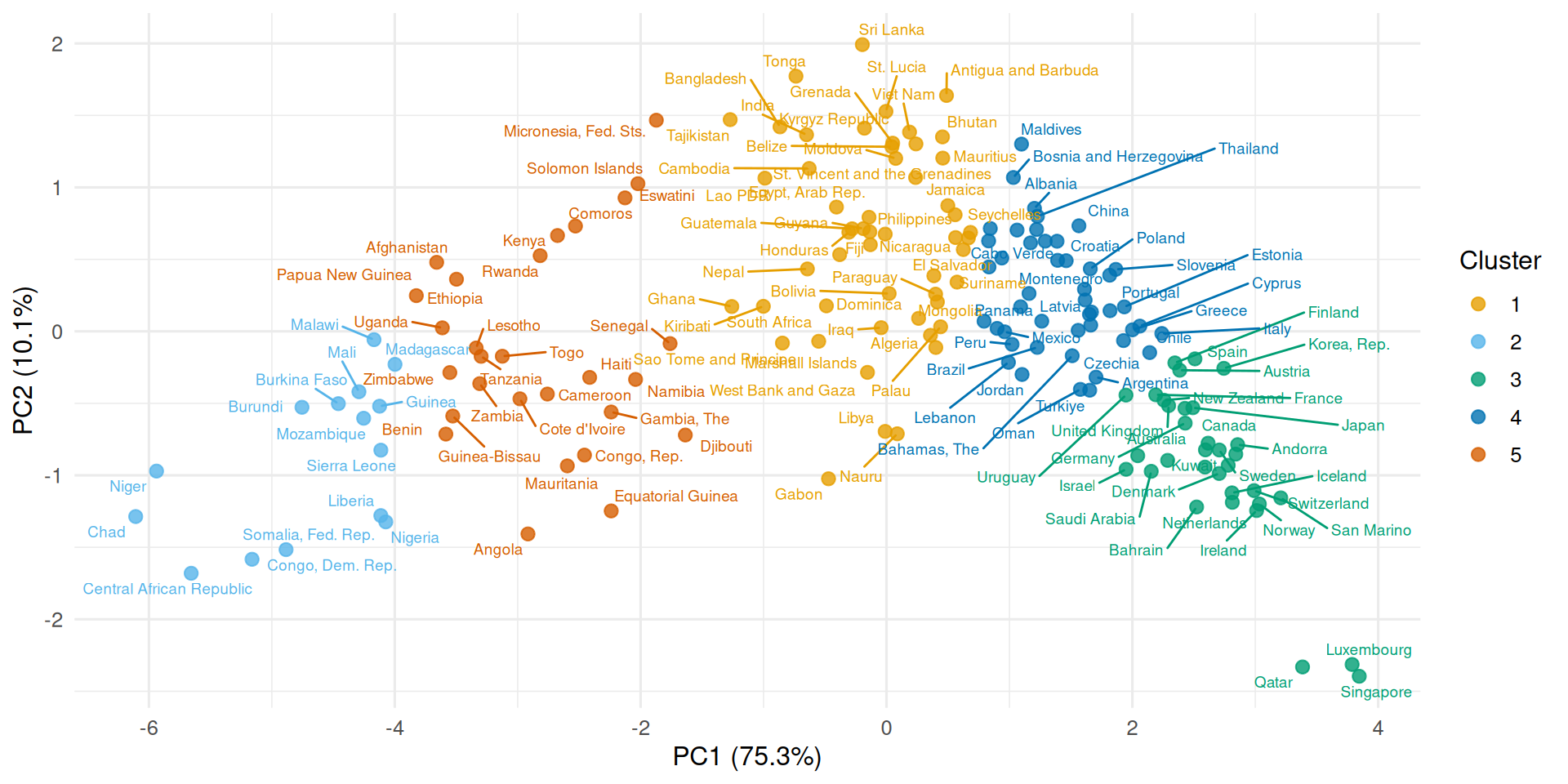
Another reason why PCA is helpful in this context is visualization: often, we want to show what our clusters look like in a visual. Our papers and screens can only accommodate two dimensions, so PCA provides a straightforward way of handling that: use PC1 and PC2 for clustering, then visualize only in those dimensions. Even if more than two dimensions were used for clustering, it would make sense to visualize it in this way. Here is an example with the World Development Indicators data:
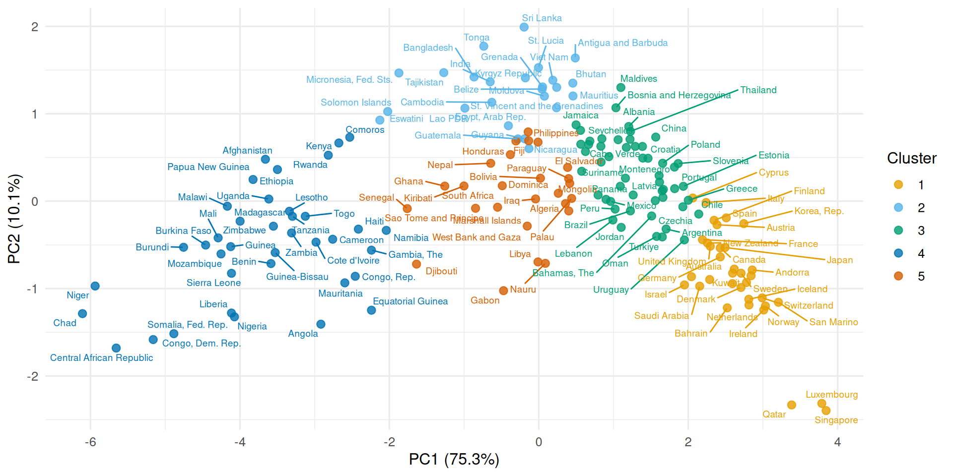
We can also cluster on more dimensions while still visualizing in two. Here we cluster on PC1, PC2, and PC3, then project the result onto the PC1–PC2 plane:
One of the great uses of PCA is as a preprocessing step for various machine learning algorithms, both supervised and unsupervised. The simple process is to apply PCA to the data; decide a number, \(M\), of the first principal components to keep for further analysis; then proceed with the remainder as you otherwise would.
There are two situations that PCA can help with: preventing overfitting and overcoming the curse of dimensionality.
One of the most fundamental problems one runs into in supervised machine learning is the problem “overfitting.” This is a big topic on its own, but we can summarize this as the algorithm trying to learn much more from the data than data of this size is able to support. Overfitting most notably happens when a model has too many parameters—it is too flexible—relative to the size of the dataset.
Say you are going to fit a linear regression, logistic regression, or another generalized linear model and you have \(p\) columns. By reducing the dimensions to \(M\), then fitting the model on the \(M\) columns, you are making the model try to learn fewer parameters and prevent overfitting.
Another way of phrasing this problem is “multicollinearity.” When a column’s information is already captured by other columns, the algorithm cannot reliably estimate coefficients for each of the variables at once. PCA detects this and consolidates all of that information into fewer columns. We then proceed with those fewer columns.
It is important to note that this is not always going to work: it depends on the extent to which lower dimensions are able to capture the important variation in the data, the dataset size, etc. The best way to proceed is to do cross-validation to decide on the \(M\).
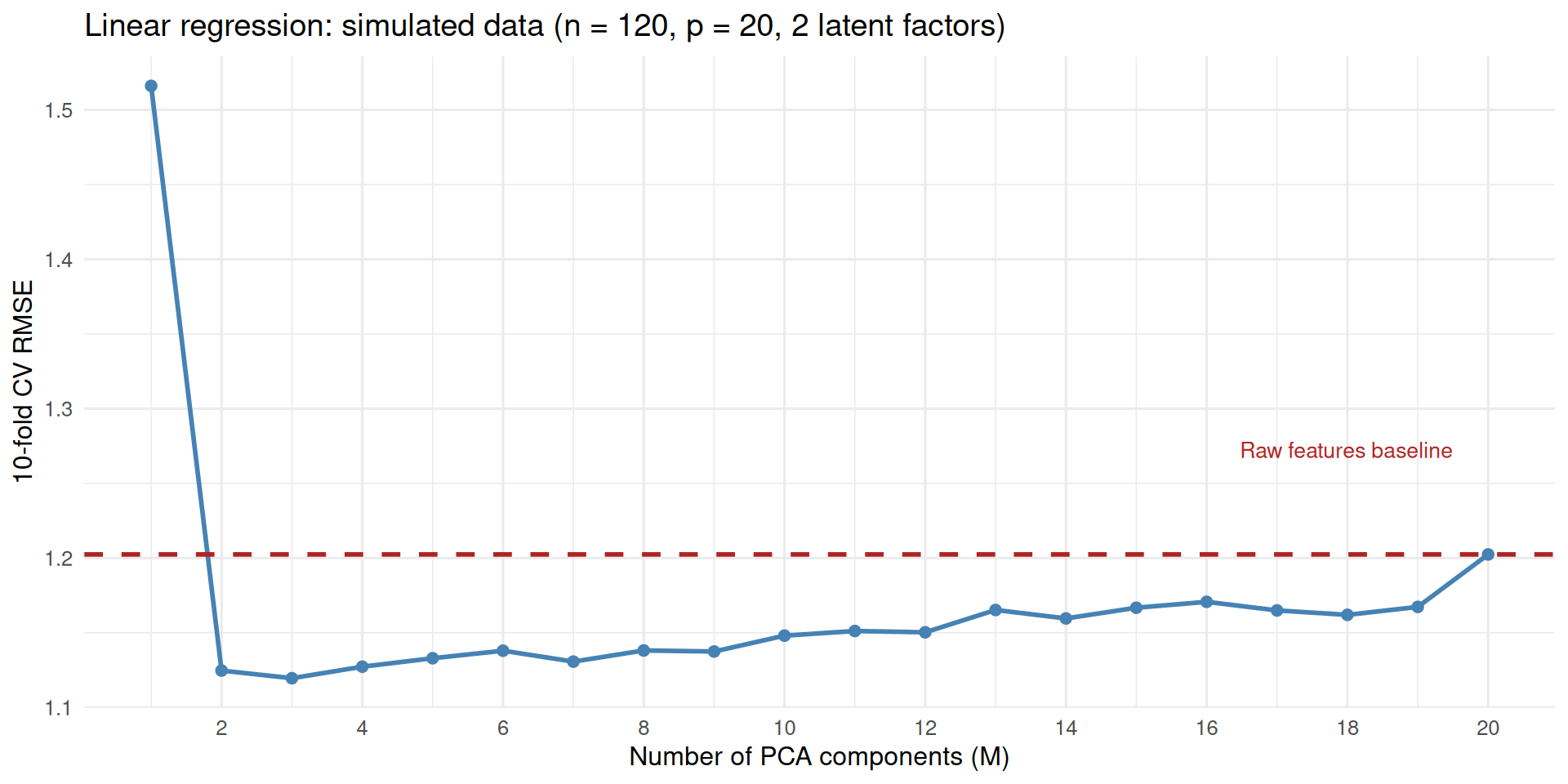
The following example makes this concrete. We simulate a dataset with \(p = 20\) highly correlated features, all generated from just 2 latent factors. We then use 10-fold cross-validation to compare linear regression on the first \(M\) PCA components against linear regression on all 20 raw features. The dashed red line is the raw-features baseline.
Show simulation and plotting
set.seed(2) # seed is 2 because the plot becomes much starker, # but the actual lesson does not change no matter the seedn_sim <-120p_sim <-20n_fac <-2F_sim <-matrix(rnorm(n_sim * n_fac), n_sim, n_fac)L_sim <-matrix(rnorm(p_sim * n_fac), p_sim, n_fac)X_sim <-scale(F_sim %*%t(L_sim) +matrix(rnorm(n_sim * p_sim, sd =0.2), n_sim, p_sim))y_sim <-3* F_sim[, 1] -2* F_sim[, 2] +rnorm(n_sim, sd =1)k_cv <-10folds <-sample(rep(1:k_cv, length.out = n_sim))fold_rmse <-function(tr_X, te_X, tr_y, te_y) { fit <-lm(tr_y ~ ., data =as.data.frame(tr_X)) pred <-predict(fit, newdata =as.data.frame(te_X))sqrt(mean((te_y - pred)^2))}rmse_pca <-sapply(1:p_sim, function(m) {mean(sapply(1:k_cv, function(k) { tr_X <- X_sim[folds != k, ]; te_X <- X_sim[folds == k, ] tr_y <- y_sim[folds != k]; te_y <- y_sim[folds == k] pca_fit <-prcomp(tr_X, scale. =FALSE)fold_rmse(pca_fit$x[, 1:m, drop =FALSE],predict(pca_fit, te_X)[, 1:m, drop =FALSE], tr_y, te_y) }))})rmse_raw <-mean(sapply(1:k_cv, function(k) {fold_rmse(X_sim[folds != k, ], X_sim[folds == k, ], y_sim[folds != k], y_sim[folds == k])}))data.frame(M =1:p_sim, RMSE = rmse_pca) |>ggplot(aes(M, RMSE)) +geom_line(color = pal$point, linewidth =1) +geom_point(color = pal$point, size =2) +geom_hline(yintercept = rmse_raw, linetype ="dashed",color = pal$accent, linewidth =1) +annotate("text", x = p_sim -0.5, y = rmse_raw +0.07,label ="Raw features baseline", color = pal$accent, hjust =1, size =3.5) +scale_x_continuous(breaks =seq(2, p_sim, by =2)) +labs(x ="Number of PCA components (M)", y ="10-fold CV RMSE",title =sprintf("Linear regression: simulated data (n = %d, p = %d, 2 latent factors)", n_sim, p_sim))
Like clustering algorithms, some supervised learning algorithms like k-Nearest Neighbors (kNN) regression and classification use distance metrics for the regression or classification task. For the same reasons as clustering algorithms (“curse of dimensionality”), PCA is helpful when doing kNN with high dimensional data. Fitting these models in lower dimensions after PCA is usually going to help them perform better. Again, cross-validation can be used to find the best number of dimensions to use.
WarningAvoid data leakage
In supervised learning applications where PCA is a preprocessing step, it is important to prevent data leakage. The correct way of doing this is to “fit” the PCA only to the training data, and use the loadings from the fitted object to transform the validation / test set to find its scores. In fact, if PCA is used for visualization or exploratory data analysis, that should only be done on the training set also.
Index Construction
Another use of PCA is for the construction of indices. In fact, we have already done it here. The biplot’s PC1 axis loads positively on income, life expectancy, internet use, electricity access, and urban population share and negatively on infant mortality and fertility—which reads naturally as a single-number summary of a country’s level of “development.” A country’s horizontal position in that plot is, in effect, its place on a crude development ranking, and we can pull that ranking out directly. In general, you may find yourself in a situation where there are multiple variables that you know from domain knowledge to roughly represent the same idea. In that case, it may be helpful to represent that information in a single column by applying PCA and taking PC1. This can be better justified if, like in our example, PC1 captures a big share of the total variance.
The result is a single number per country—here are the top and bottom of the ranking:
Why is this desirable? Whenever the goal of a study is inference about the “effect” of a treatment, it is useful to have one variable that can represent different levels of that treatment. When you have multiple variables, you cannot include all of them in the same model: they represent the same idea and you cannot meaningfully hold one constant and let the others change—this would be both difficult to estimate and impossible to interpret. The reasonable alternative is to fit separate models with each alternative measurement, but that becomes difficult if there are many variables you are considering.
A second reason why this type of index construction helps in inferential models is related to the reason why PCA can help prevent overfitting: you concentrate the strongest signals in one column and get rid of the noise. Imagine a survey setting where people have answered multiple questions about various aspects of the same concept, religiosity, such as (a) How important is God in your life?, (b) How frequently do you attend religious services?, (c) My partner has to be the same religion as me (agreement levels on Likert scale), (d) Church and state should be separate (agreement on Likert scale). It is relatively easier for individual people to misunderstand a question, be distracted, or falsify preferences for some questions due to social desirability bias. But it is going to be a lot less likely for them to do this over multiple questions. By aggregating the signal that comes from multiple questions, we reduce the noise and construct one strong signal.
Examples of situations where aggregating many dimensions to construct a single index are many, especially for hard to measure, abstract social science concepts. Some examples include measurements of judicial independence, democraticness, or freedom of press at the country level; political ideology of legislators; socioeconomic status or levels of racial prejudice in respondents, and so on.
Filmer and Pritchett (2001) construct a wealth index for Indian households using 21 separate yes/no indicators: owns a clock, owns a bicycle, has a flush toilet, cooks with biomass, and so on. Each one is a noisy, partial signal of how well-off a household is. They use PCA to collapse those into a single number that can represent wealth and allow them to say “this household is richer than this other household.” One reason they cite is that they want to use wealth as a control variable in regression so they need a single variable. Another important practical problem that PCA solves for them is the question of weights: how do you combine 21 items into a single index for wealth? Equal weights are arbitrary. They could use how much each item costs, but that’s not in the data. PCA provides a principled and automatic way of assigning weights to each dimension.
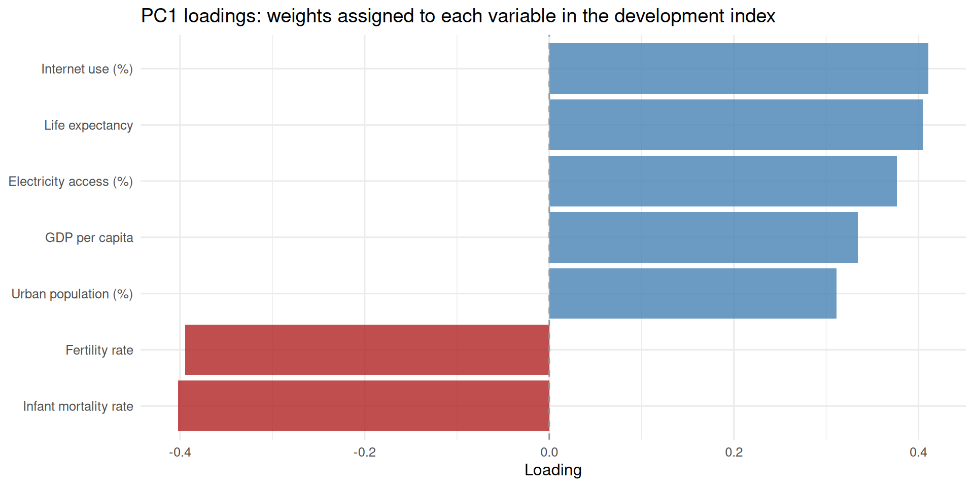
Here is how both of those things look in our World Bank data—what weights each variable receives and where each country ends up.
Show code for plotting
var_labels <-c(fertility_rate ="Fertility rate",gdp_per_capita ="GDP per capita",infant_mortality_rate ="Infant mortality rate",life_expectancy ="Life expectancy",pct_access_electricity ="Electricity access (%)",pct_urban ="Urban population (%)",pct_using_internet ="Internet use (%)")loadings_df <-data.frame(variable = var_labels[rownames(pca$rotation)],loading = pca$rotation[, 1])ggplot(loadings_df, aes(x = loading, y =reorder(variable, loading),fill = loading >0)) +geom_col(alpha =0.8, show.legend =FALSE) +scale_fill_manual(values =c("FALSE"= pal$accent, "TRUE"= pal$point)) +geom_vline(xintercept =0, linetype ="dashed", color = pal$neutral) +labs(title ="PC1 loadings: weights assigned to each variable in the development index",x ="Loading",y =NULL )
Like with all different uses of PCA, this is not a situation where PCA is the only feasible solution. A common way of constructing indices from existing variables is factor analysis. But PCA is definitely one good and quick way of doing it.
Compare Effective Number of Dimensions
Another great use of PCA is as a measurement of the extent to which some data can be represented in lower dimensions. A good proxy for this is the share of the variance captured by the first principal component. A more sophisticated analysis could treat this as a measurement of inequality and construct a version of the Gini coefficient or Herfindahl-Hirschman Index (HHI) using the variance explained values for each principal component, so that not just concentration on the first principal component but the overall distribution is taken into account.
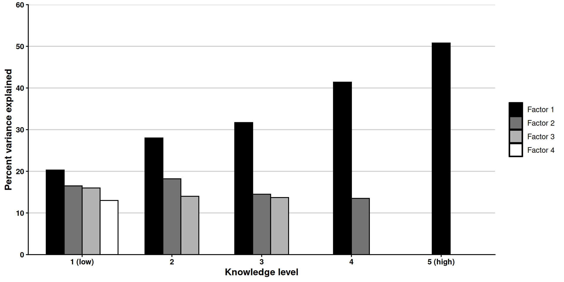
Michaud et al. (2009) provide a good example of this. They study the extent to which two worldviews—egalitarianism and individualism—are understood as the opposite ends of a single spectrum or not. To this end, they look at results from a survey where participants were asked to indicate their level of agreement with eight statements—four of them indicators of egalitarian values and four of them of individualistic values.
They then segment respondents based on their political knowledge, measured with a series of questions about contemporary US politics (for example, “Do you happen to know which party has the most members in the House of Representatives right now?”) They do PCA on the survey data that comes from different segments of the respondents, showing that the first principal component explains about 50% of the variance for people with the highest levels of political knowledge, but it explains 20% of the variance for those with the lowest levels of political knowledge.
This is what the central finding in Michaud et al. (2009) looks like:
Show code for plotting
# This plot intentionally departs from the post's shared style: its grayscale# fills and theme_classic reproduce the look of the original publication figure.michaud <-data.frame(knowledge =factor(rep(c("1 (low)", "2", "3", "4", "5 (high)"), times =c(4, 3, 3, 2, 1)),levels =c("1 (low)", "2", "3", "4", "5 (high)")),factor =c("Factor 1", "Factor 2", "Factor 3", "Factor 4","Factor 1", "Factor 2", "Factor 3","Factor 1", "Factor 2", "Factor 3","Factor 1", "Factor 2","Factor 1"),variance =c(20.3, 16.5, 16.0, 13.0,28.0, 18.2, 14.0,31.7, 14.5, 13.7,41.4, 13.5,50.8))michaud$factor <-factor(michaud$factor,levels =c("Factor 1", "Factor 2", "Factor 3", "Factor 4"))ggplot(michaud, aes(x = knowledge, y = variance, fill = factor)) +geom_col(position =position_dodge2(preserve ="single", padding =0),color ="black", width =0.8) +scale_fill_manual(values =c("Factor 1"="black","Factor 2"="gray45","Factor 3"="gray70","Factor 4"="white")) +scale_y_continuous(limits =c(0, 60), breaks =seq(0, 60, 10),expand =c(0, 0)) +labs(x ="Knowledge level", y ="Percent variance explained", fill =NULL) +theme_classic(base_size =12) +theme(axis.title =element_text(face ="bold"),axis.text =element_text(color ="black", face ="bold"),legend.key =element_rect(color ="black"),legend.position ="right",panel.grid.major.y =element_line(color ="gray80") )
It seems like those with high levels of political knowledge tend to see each question as a proxy for where they place themselves in the political spectrum, but those with lower levels of political knowledge just perceive each question as distinct questions that they independently answer based on their value judgments for that question. Note that calling the principal components “factors” and plotting fewer of the principal components as the variance in PC1 increases is the paper’s choice—this is a close reproduction.
This is really a cool application, one that can be easily applied in other contexts. For example, how many ideological dimensions are people’s worldviews shaped by in two-party vs multi-party systems; worldview differences in post-Soviet vs Western Europe, and so on.
Matrix Completion
Another use of PCA is matrix completion. Matrix completion algorithms are useful in at least two important ways: (1) matrix completion can be a task of interest in its own right—for example, in recommendation systems, where rows correspond to users, columns to movies, and each user has rated some movies but not others; here, predicting the missing values amounts to predicting how much a user would like a given movie; (2) matrix completion can be used to impute missing values in a data matrix for downstream use, for example in a supervised learning task with missing values for predictors.
Every matrix completion algorithm relies on one important assumption: that missing values are somewhat predictable from non-missing values in other columns. What does it mean for columns to be able to predict each other? It means that they have an underlying lower dimensional structure—exactly what PCA specializes in representing. To the extent that this assumption holds, matrix completion will work.
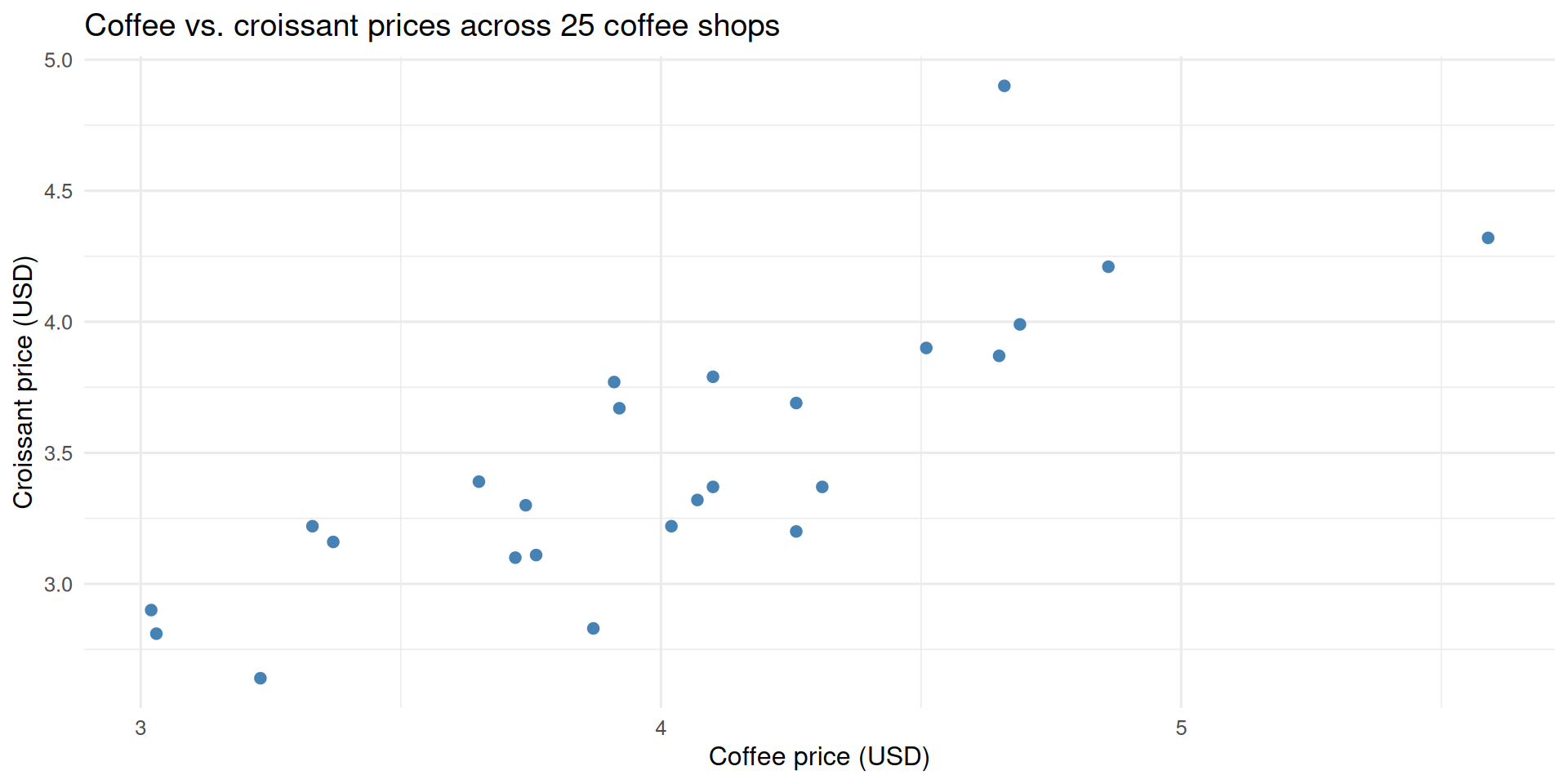
Consider a dataset where we record the price of a coffee and the price of a croissant at 25 different coffee shops. These two prices will be correlated—more expensive places will tend to charge more for both—but not perfectly. Unlike a unit-conversion (say, pounds to kilograms), the relationship is real but noisy.
ggplot(shops, aes(coffee, croissant)) +geom_point(color = pal$point, size =2) +labs(x ="Coffee price (USD)", y ="Croissant price (USD)",title ="Coffee vs. croissant prices across 25 coffee shops")
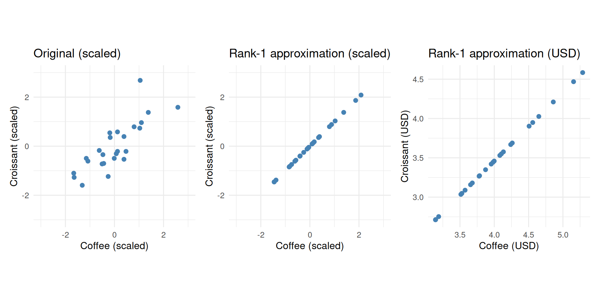
Recall that PCA rotates the data into PC space by multiplying by the rotation matrix; multiplying by its transpose brings the data back. If we set PC2 to zero before rotating back, we get the best rank-1 approximation of the data. In general, we can rotate back the \(M\) dimensions of the transformed data where \(M < p\) to get the best \(M\) dimensional approximation to the original data—“best” meaning it minimizes the sum of squared differences between each cell of the original matrix and the corresponding cell of the reconstructed matrix. In this specific case, the two original columns collapse onto a single line. The reconstruction recovers distinct coffee and croissant prices in the original axes.
The middle plot shows the rank-1 approximation in the scaled space—all points on a line. The right-hand plot multiplies each column back by its original standard deviation and adds its original mean, recovering interpretable dollar prices that still lie on that same line.
Why would you want to do a low rank approximation to the original data? Imagine that for some coffee shops the price of coffee is missing and for others the price of croissant is missing. PCA reveals the fundamental relationship between the two, the extent to which they vary together, and consolidates that information in PC1. For any coffee shop, if we know their coffee price, we can use that single-axis to approximately recover their croissant value and vice versa—assuming that the overall relationship between the coffee and croissant prices in other coffee shops holds for those with missing values too.
James et al. (2021) provide the following simple algorithm:
Initialize each missing value with its column mean.
Fit a rank-\(M\) PCA approximation to the filled matrix.
Replace each missing entry with its rank-\(M\) reconstruction.
Repeat steps 2–3 until the change in imputed values falls below a threshold.
Let’s randomly remove some of the values from our example and use the algorithm to recover them.
impute_pca <-function(X, M =1, thresh =1e-7, max_iter =100) {# record which cells are missing so we only ever update those na_mask <-is.na(X) X_filled <- X# step 1: initialize each missing value with its column meanfor (j inseq_len(ncol(X))) X_filled[is.na(X[, j]), j] <-mean(X[, j], na.rm =TRUE) prev_vals <- X_filled[na_mask]for (iter inseq_len(max_iter)) {# step 2: fit PCA to the current (fully filled) matrix fit <-prcomp(X_filled, center =TRUE, scale. =FALSE)# step 3: reconstruct via rank-M approximation (scores × loadings^T)# prcomp centers the data internally, so we add the center back X_approx <- fit$x[, seq_len(M), drop =FALSE] %*%t(fit$rotation[, seq_len(M), drop =FALSE]) X_approx <-sweep(X_approx, 2, fit$center, "+")# step 4: update only the originally missing cells X_filled[na_mask] <- X_approx[na_mask]# stop when the imputed values change by less than thresh change <-mean((X_filled[na_mask] - prev_vals)^2)if (change < thresh) break prev_vals <- X_filled[na_mask] }list(imputed = X_filled, iters = iter)}
result <-impute_pca(shops_missing, M =1)cat("Converged in", result$iters, "iterations\n")
Converged in 17 iterations
We can compare the imputed values against the true (held-out) values:
Show code for comparison table
na_mask <-is.na(shops_missing)true_scaled <-as.matrix(shops_scaled)[na_mask]imp_scaled <- result$imputed[na_mask]# which column does each missing value belong to?col_idx <-col(shops_missing)[na_mask]true_usd <- true_scaled * original_sds[col_idx] + original_means[col_idx]imp_usd <- imp_scaled * original_sds[col_idx] + original_means[col_idx]data.frame(true_scaled =round(true_scaled, 3),imputed_scaled =round(imp_scaled, 3),true_usd =round(true_usd, 2),imputed_usd =round(imp_usd, 2)) |>kable(col.names =c("True (scaled)", "Imputed (scaled)", "True (USD)", "Imputed (USD)"),caption ="Imputed vs. held-out true values for the removed cells" )
Imputed vs. held-out true values for the removed cells
True (scaled)
Imputed (scaled)
True (USD)
Imputed (USD)
-0.009
-0.587
4.02
3.67
-0.438
-0.853
3.76
3.51
0.124
0.791
4.10
4.50
1.377
1.043
4.21
4.03
2.683
0.784
4.90
3.90
-1.271
-1.322
2.81
2.78
-0.306
0.022
3.32
3.49
-0.534
0.267
3.20
3.62
In short, if we have low rank data, which means a lower dimensional representation can capture all or most of the variation in the data, PCA can do a good job of recovering missing values using the iterative algorithm. Depending on the application, one can once again use an experimental methodology like cross-validation to assess how many dimensions, \(M\), work well on the task and to also assess PCA against alternative forms of missing value imputation.
Notes
This post covers five cool uses of PCA that I encountered in research and teaching, with a review section in the beginning. I used Claude Code for writing some of the code, especially for most of the plotting, and in some sections to smooth out my language and correct grammar errors. I am responsible for any mistakes or inaccuracies.
Filmer, Deon, and Lant H Pritchett. 2001. “Estimating Wealth Effects Without Expenditure Data—or Tears: An Application to Educational Enrollments in States of India.”Demography 38 (1): 115–32.
Grootendorst, Maarten. 2022. “BERTopic: Neural Topic Modeling with a Class-Based TF-IDF Procedure.”arXiv Preprint arXiv:2203.05794.
James, Gareth, Daniela Witten, Trevor Hastie, and Robert Tibshirani. 2021. An Introduction to Statistical Learning: With Applications in r. 2nd ed. Springer Texts in Statistics. Springer. https://www.statlearning.com.
Michaud, Kristy EH, Juliet E Carlisle, and Eric RAN Smith. 2009. “The Relationship Between Cultural Values and Political Ideology, and the Role of Political Knowledge.”Political Psychology 30 (1): 27–42.
Nakka, Nitheesha, Omer F. Yalcin, Bruce A. Desmarais, Sarah Rajtmajer, and Burt Monroe. 2025. The Study of Short Texts in Digital Politics: Document Aggregation for Topic Modeling. https://arxiv.org/abs/2503.05065.